Subsetting a Cube#
The Loading Iris Cubes section of the user guide showed how to load data into multidimensional Iris cubes. However it is often necessary to reduce the dimensionality of a cube down to something more appropriate and/or manageable, or only examine and analyse a subset of data in a dimension.
Iris provides several ways of reducing both the amount of data and/or the number of dimensions in your cube depending on the circumstance. In all cases the subset of a valid cube is itself a valid cube.
See also
- Relevant gallery examples:
Fitting a Polynomial (Slices)
Colouring Anomaly Data With Logarithmic Scaling (Extraction)
Cube Extraction#
A subset of a cube can be “extracted” from a multi-dimensional cube in order to reduce its dimensionality:
>>> import iris
>>> filename = iris.sample_data_path('space_weather.nc')
>>> cube = iris.load_cube(filename, 'electron density')
>>> equator_slice = cube.extract(iris.Constraint(grid_latitude=0))
>>> print(equator_slice)
electron density / (1E11 e/m^3)     (height: 29; grid_longitude: 31)
    Dimension coordinates:
        height                             x                   -
        grid_longitude                     -                   x
    Auxiliary coordinates:
        latitude                           -                   x
        longitude                          -                   x
    Scalar coordinates:
        grid_latitude               0.0 degrees
    Attributes:
        Conventions                 'CF-1.5'
In this example we start with a 3 dimensional cube, with dimensions of height, grid_latitude and grid_longitude,
and use iris.Constraint to extract every point where the latitude is 0, resulting in a 2d cube with axes of height and grid_longitude.
Warning
Caution is required when using equality constraints with floating point coordinates such as grid_latitude.
Printing the points of a coordinate does not necessarily show the full precision of the underlying number and it
is very easy to return no matches to a constraint when one was expected.
This can be avoided by using a function as the argument to the constraint:
def near_zero(cell):
   """Returns true if the cell is between -0.1 and 0.1."""
   return -0.1 < cell < 0.1

equator_constraint = iris.Constraint(grid_latitude=near_zero)
Often you will see this construct in shorthand using a lambda function definition:
equator_constraint = iris.Constraint(grid_latitude=lambda cell: -0.1 < cell < 0.1)
The extract method could be applied again to the equator_slice cube to get a further subset.
For example to get a height of 9000 metres at the equator the following line extends the previous example:
equator_height_9km_slice = equator_slice.extract(iris.Constraint(height=9000))
print(equator_height_9km_slice)
The two steps required to get height of 9000 m at the equator can be simplified into a single constraint:
equator_height_9km_slice = cube.extract(iris.Constraint(grid_latitude=0, height=9000))
print(equator_height_9km_slice)
Alternatively, constraints can be combined using &:
cube = iris.load_cube(filename, 'electron density')
equator_constraint = iris.Constraint(grid_latitude=0)
height_constraint = iris.Constraint(height=9000)
equator_height_9km_slice = cube.extract(equator_constraint & height_constraint)
Note
Whilst & is supported, the | that might reasonably be expected is
not. Explanation as to why is in the iris.Constraint reference
documentation.
For an example of constraining to multiple ranges of the same coordinate to
generate one cube, see the iris.Constraint reference documentation.
A common requirement is to limit the value of a coordinate to a specific range, this can be achieved by passing the constraint a function:
def below_9km(cell):
    # return True or False as to whether the cell in question should be kept
    return cell <= 9000

cube = iris.load_cube(filename, 'electron density')
height_below_9km = iris.Constraint(height=below_9km)
below_9km_slice = cube.extract(height_below_9km)
As we saw in Loading Iris Cubes the result of iris.load() is a CubeList.
The extract method also exists on a CubeList and behaves in exactly the
same way as loading with constraints:
>>> import iris
>>> air_temp_and_fp_6 = iris.Constraint('air_potential_temperature', forecast_period=6)
>>> level_10 = iris.Constraint(model_level_number=10)
>>> filename = iris.sample_data_path('uk_hires.pp')
>>> cubes = iris.load(filename).extract(air_temp_and_fp_6 & level_10)
>>> print(cubes)
0: air_potential_temperature / (K)     (grid_latitude: 204; grid_longitude: 187)
>>> print(cubes[0])
air_potential_temperature / (K)     (grid_latitude: 204; grid_longitude: 187)
    Dimension coordinates:
        grid_latitude                             x                    -
        grid_longitude                            -                    x
    Auxiliary coordinates:
        surface_altitude                          x                    x
    Derived coordinates:
        altitude                                  x                    x
    Scalar coordinates:
        forecast_period             6.0 hours
        forecast_reference_time     2009-11-19 04:00:00
        level_height                395.0 m, bound=(360.0, 433.3332) m
        model_level_number          10
        sigma                       0.9549927, bound=(0.9589389, 0.95068014)
        time                        2009-11-19 10:00:00
    Attributes:
        STASH                       m01s00i004
        source                      'Data from Met Office Unified Model'
        um_version                  '7.3'
Cube attributes can also be part of the constraint criteria. Supposing a
cube attribute of STASH existed, as is the case when loading PP files,
then specific STASH codes can be filtered:
filename = iris.sample_data_path('uk_hires.pp')
level_10_with_stash = iris.AttributeConstraint(STASH='m01s00i004') & iris.Constraint(model_level_number=10)
cubes = iris.load(filename).extract(level_10_with_stash)
See also
For advanced usage there are further examples in the
iris.Constraint reference documentation.
Constraining a Circular Coordinate Across its Boundary#
Occasionally you may need to constrain your cube with a region that crosses the boundary of a circular coordinate (this is often the meridian or the dateline / antimeridian). An example use-case of this is to extract the entire Pacific Ocean from a cube whose longitudes are bounded by the dateline.
This functionality cannot be provided reliably using constraints. Instead you should use the
functionality provided by cube.intersection
to extract this region.
Constraining on Time#
Iris follows NetCDF-CF rules in representing time coordinate values as normalised, purely numeric, values which are normalised by the calendar specified in the coordinate’s units (e.g. “days since 1970-01-01”). However, when constraining by time we usually want to test calendar-related aspects such as hours of the day or months of the year, so Iris provides special features to facilitate this.
Firstly, when Iris evaluates iris.Constraint expressions, it will convert
time-coordinate values (points and bounds) from numbers into datetime-like
objects for ease of calendar-based testing.
>>> filename = iris.sample_data_path('uk_hires.pp')
>>> cube_all = iris.load_cube(filename, 'air_potential_temperature')
>>> print('All times :\n' + str(cube_all.coord('time')))
All times :
DimCoord :  time / (hours since 1970-01-01 00:00:00, standard calendar)
    points: [2009-11-19 10:00:00, 2009-11-19 11:00:00, 2009-11-19 12:00:00]
    shape: (3,)
    dtype: float64
    standard_name: 'time'
>>> # Define a function which accepts a datetime as its argument (this is simplified in later examples).
>>> hour_11 = iris.Constraint(time=lambda cell: cell.point.hour == 11)
>>> cube_11 = cube_all.extract(hour_11)
>>> print('Selected times :\n' + str(cube_11.coord('time')))
Selected times :
DimCoord :  time / (hours since 1970-01-01 00:00:00, standard calendar)
    points: [2009-11-19 11:00:00]
    shape: (1,)
    dtype: float64
    standard_name: 'time'
Secondly, the iris.time module provides flexible time comparison
facilities. An iris.time.PartialDateTime object can be compared to
objects such as datetime.datetime instances, and this comparison will
then test only those ‘aspects’ which the PartialDateTime instance defines:
>>> import datetime
>>> from iris.time import PartialDateTime
>>> dt = datetime.datetime(2011, 3, 7)
>>> print(dt > PartialDateTime(year=2010, month=6))
True
>>> print(dt > PartialDateTime(month=6))
False
These two facilities can be combined to provide straightforward calendar-based time selections when loading or extracting data.
The previous constraint example can now be written as:
>>> the_11th_hour = iris.Constraint(time=iris.time.PartialDateTime(hour=11))
>>> print(iris.load_cube(
...     iris.sample_data_path('uk_hires.pp'),
...    'air_potential_temperature' & the_11th_hour).coord('time'))
DimCoord :  time / (hours since 1970-01-01 00:00:00, standard calendar)
    points: [2009-11-19 11:00:00]
    shape: (1,)
    dtype: float64
    standard_name: 'time'
It is common that a cube will need to be constrained between two given dates. In the following example we construct a time sequence representing the first day of every week for many years:
>>> print(long_ts.coord('time'))
DimCoord :  time / (days since 2007-04-09, standard calendar)
    points: [
        2007-04-09 00:00:00, 2007-04-16 00:00:00, ...,
        2010-02-08 00:00:00, 2010-02-15 00:00:00]
    shape: (150,)
    dtype: int64
    standard_name: 'time'
Given two dates in datetime format, we can select all points between them.
Instead of constraining at loaded time, we already have the time coord so
we constrain that coord using iris.cube.Cube.extract
>>> d1 = datetime.datetime.strptime('20070715T0000Z', '%Y%m%dT%H%MZ')
>>> d2 = datetime.datetime.strptime('20070825T0000Z', '%Y%m%dT%H%MZ')
>>> st_swithuns_daterange_07 = iris.Constraint(
...     time=lambda cell: d1 <= cell.point < d2)
>>> within_st_swithuns_07 = long_ts.extract(st_swithuns_daterange_07)
>>> print(within_st_swithuns_07.coord('time'))
DimCoord :  time / (days since 2007-04-09, standard calendar)
    points: [
        2007-07-16 00:00:00, 2007-07-23 00:00:00, 2007-07-30 00:00:00,
        2007-08-06 00:00:00, 2007-08-13 00:00:00, 2007-08-20 00:00:00]
    shape: (6,)
    dtype: int64
    standard_name: 'time'
Alternatively, we may rewrite this using iris.time.PartialDateTime
objects.
>>> pdt1 = PartialDateTime(year=2007, month=7, day=15)
>>> pdt2 = PartialDateTime(year=2007, month=8, day=25)
>>> st_swithuns_daterange_07 = iris.Constraint(
...     time=lambda cell: pdt1 <= cell.point < pdt2)
>>> within_st_swithuns_07 = long_ts.extract(st_swithuns_daterange_07)
>>> print(within_st_swithuns_07.coord('time'))
DimCoord :  time / (days since 2007-04-09, standard calendar)
    points: [
        2007-07-16 00:00:00, 2007-07-23 00:00:00, 2007-07-30 00:00:00,
        2007-08-06 00:00:00, 2007-08-13 00:00:00, 2007-08-20 00:00:00]
    shape: (6,)
    dtype: int64
    standard_name: 'time'
A more complex example might require selecting points over an annually repeating date range. We can select points within a certain part of the year, in this case between the 15th of July through to the 25th of August. By making use of PartialDateTime this becomes simple:
>>> st_swithuns_daterange = iris.Constraint(
...     time=lambda cell: PartialDateTime(month=7, day=15) <= cell.point < PartialDateTime(month=8, day=25))
>>> within_st_swithuns = long_ts.extract(st_swithuns_daterange)
...
>>> # Note: using summary(max_values) to show more of the points
>>> print(within_st_swithuns.coord('time').summary(max_values=100))
DimCoord :  time / (days since 2007-04-09, standard calendar)
    points: [
        2007-07-16 00:00:00, 2007-07-23 00:00:00, 2007-07-30 00:00:00,
        2007-08-06 00:00:00, 2007-08-13 00:00:00, 2007-08-20 00:00:00,
        2008-07-21 00:00:00, 2008-07-28 00:00:00, 2008-08-04 00:00:00,
        2008-08-11 00:00:00, 2008-08-18 00:00:00, 2009-07-20 00:00:00,
        2009-07-27 00:00:00, 2009-08-03 00:00:00, 2009-08-10 00:00:00,
        2009-08-17 00:00:00, 2009-08-24 00:00:00]
    shape: (17,)
    dtype: int64
    standard_name: 'time'
Notice how the dates printed are between the range specified in the st_swithuns_daterange
and that they span multiple years.
The above examples involve constraining on the points of the time coordinate. Constraining on bounds can be done in the following way:
filename = iris.sample_data_path('ostia_monthly.nc')
cube = iris.load_cube(filename, 'surface_temperature')
dtmin = datetime.datetime(2008, 1, 1)
cube.extract(iris.Constraint(time = lambda cell: any(bound > dtmin for bound in cell.bound)))
The above example constrains to cells where either the upper or lower bound occur after 1st January 2008.
Cube Masking#
Masking a cube allows you to hide unwanted data points without changing the shape or size of the cube. This can be achieved by two methods:
Masking a cube using a boolean mask array via
iris.util.mask_cube().Masking a cube using a shapefile via
iris.util.mask_cube_from_shape().
Masking a cube using a boolean mask array#
The iris.util.mask_cube() function allows you to mask unwanted data points
in a cube using a boolean mask array. The mask array must have the same shape as
the data array in the cube, with True values indicating points to be masked.
For example, the mask could be based on a threshold value. In the following example we mask all points in a cube where the air potential temperature is greater than 290 K.
>>> filename = iris.sample_data_path('uk_hires.pp')
>>> cube_temp = iris.load_cube(filename, 'air_potential_temperature')
>>> print(cube_temp.summary(shorten=True))
air_potential_temperature / (K)     (time: 3; model_level_number: 7; grid_latitude: 204; grid_longitude: 187)
>>> type(cube_temp.data)
<class 'numpy.ndarray'>
Note that this example cube has 4 dimensions: time and model level number in
addition to grid latitude, and grid longitude. The data array associated with
the cube is a regular numpy.ndarray.
We can build a boolean mask array by applying a condition to the cube’s data array:
>>> mask = cube_temp.data > 290
>>> cube_masked = iris.util.mask_cube(cube_temp, mask)
>>> print(cube_masked.summary(shorten=True))
air_potential_temperature / (K)     (time: 3; model_level_number: 7; grid_latitude: 204; grid_longitude: 187)
>>> type(cube_masked.data)
<class 'numpy.ma.MaskedArray'>
The masked cube will have the same shape and coordinates as the original cube,
but the data array now includes an associated boolean mask, and the cube’s
data property is now a numpy.ma.MaskedArray.
Masking from a shapefile#
Often we want to perform some kind of analysis over a complex geographical feature e.g.,
over only land/sea points
over a continent, country, or list of countries
over a river watershed or lake basin
over states or administrative regions of a country
extract data along the trajectory of a storm track
extract data at specific points of interest such as cities or weather stations
These geographical features can often be described by ESRI Shapefiles. Shapefiles are a file format first developed for GIS software in the 1990s, and Natural Earth maintain a large freely usable database of shapefiles of many geographical and political divisions, accessible via cartopy. Users may also provide or create their own custom shapefiles for cartopy to load, or or any other source that can be interpreted as a shapely.Geometry object, such as shapes encoded in a geoJSON or KML file.
The iris.util.mask_cube_from_shape() function facilitates cube masking
from shapefiles. Once a shape is loaded as a shapely.Geometry, and passed to
the function, any data outside the bounds of the shape geometry is masked.
Important
For best masking results, both the cube and masking shape (geometry)
should have a coordinate reference system (CRS) defined. Note that the CRS of
the masking geometry must be provided explicitly to iris.util.mask_cube_from_shape()
(via the shape_crs keyword argument), whereas the iris.cube.Cube
CRS is read from the cube itself.
The cube must have a iris.coords.Coord.coord_system defined
otherwise an error will be raised.
Note
Because shape vectors are inherently Cartesian in nature, they contain no inherent understanding of the spherical geometry underpinning geographic coordinate systems. For this reason, shapefiles or shape vectors that cross the antimeridian or poles are not supported by this function to avoid unexpected masking behaviour.
For shapes that do cross these boundaries, this function expects the user to undertake fixes upstream of Iris, using tools like GDAL or antimeridian to ensure correct geometry wrapping.
As an introductory example, we load a shapefile of country borders for Brazil
from Natural Earth via the Cartopy_shapereader. The .geometry attribute
of the records in the reader contain the Shapely polygon we’re interested in.
They contain the coordinates that define the polygon being masked under the
WGS84 coordinate system. We pass this to the iris.util.mask_cube_from_shape
function and this returns a copy of the cube with a numpy.masked_array
as the data payload, where the data outside the shape is hidden by the masked
array.
"""Global cube masked to Brazil and plotted with quickplot."""

import cartopy.io.shapereader as shpreader
import matplotlib.pyplot as plt

import iris
import iris.quickplot as qplt
from iris.util import mask_cube_from_shape

country_shp_reader = shpreader.Reader(
    shpreader.natural_earth(
        resolution="110m", category="cultural", name="admin_0_countries"
    )
)
brazil_shp = [
    country.geometry
    for country in country_shp_reader.records()
    if "Brazil" in country.attributes["NAME_LONG"]
][0]

cube = iris.load_cube(iris.sample_data_path("air_temp.pp"))
brazil_cube = mask_cube_from_shape(cube=cube, shape=brazil_shp)

qplt.pcolormesh(brazil_cube)
plt.show()
(Source code, png)
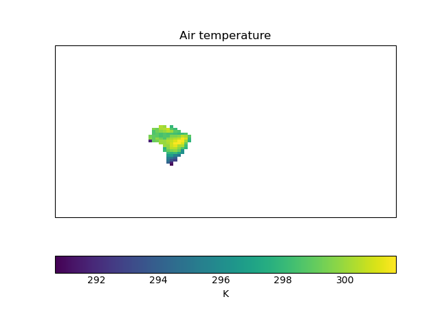

We can see that the dimensions of the cube haven’t changed - the plot still has a global extent. But only the data over Brazil is plotted - the rest has been masked out.
Important
Because we do not explicitly pass a CRS for the shape geometry to
iris.util.mask_cube_from_shape(), the function assumes the geometry
has the same CRS as the cube.
However, a iris.cube.Cube and Shapely geometry do not need to have
the same CRS, as long as both have a CRS defined. Where the CRS of the
iris.cube.Cube and geometry differ, iris.util.mask_cube_from_shape()
will reproject the geometry (via GDAL) onto the cube’s CRS prior to masking.
The masked cube will be returned in the same CRS as the input cube.
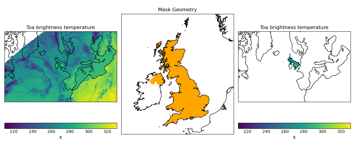
In the following example, we load a cube containing satellite derived temperature data in a stereographic projection (with projected coordinates with units of metres), and mask it to only show data over the United Kingdom, based on a shapefile of the UK boundary defined in WGS84 lat-lon coordinates.
"""Masking data with a stereographic projection and plotted with quickplot."""

import cartopy.crs as ccrs
import cartopy.io.shapereader as shpreader
import matplotlib.pyplot as plt

import iris
import iris.quickplot as qplt
from iris.util import mask_cube_from_shape

# Define WGS84 coordinate reference system
wgs84 = ccrs.PlateCarree(globe=ccrs.Globe(ellipse="WGS84"))

country_shp_reader = shpreader.Reader(
    shpreader.natural_earth(
        resolution="10m", category="cultural", name="admin_0_countries"
    )
)
uk_shp = [
    country.geometry
    for country in country_shp_reader.records()
    if "United Kingdom" in country.attributes["NAME_LONG"]
][0]

cube = iris.load_cube(iris.sample_data_path("toa_brightness_stereographic.nc"))
uk_cube = mask_cube_from_shape(cube=cube, shape=uk_shp, shape_crs=wgs84)

plt.figure(figsize=(12, 5))
# Plot #1: original data
ax = plt.subplot(131)
qplt.pcolormesh(cube, vmin=210, vmax=330)
plt.gca().coastlines()

# Plot #2: UK geometry
ax = plt.subplot(132, title="Mask Geometry", projection=ccrs.Orthographic(-5, 45))
ax.set_extent([-12, 5, 49, 61])
ax.add_geometries(
    [
        uk_shp,
    ],
    crs=wgs84,
    edgecolor="None",
    facecolor="orange",
)
plt.gca().coastlines()

# Plot #3 masked data
ax = plt.subplot(133)
qplt.pcolormesh(uk_cube, vmin=210, vmax=330)
plt.gca().coastlines()

plt.tight_layout()
plt.show()
(Source code, png)
Cube Iteration#
It is not possible to directly iterate over an Iris cube. That is, you cannot use code such as
for x in cube:. However, you can iterate over cube slices, as this section details.
A useful way of dealing with a Cube in its entirety is by iterating over its layers or slices. For example, to deal with a 3 dimensional cube (z,y,x) you could iterate over all 2 dimensional slices in y and x which make up the full 3d cube.:
import iris
filename = iris.sample_data_path('hybrid_height.nc')
cube = iris.load_cube(filename)
print(cube)
for yx_slice in cube.slices(['grid_latitude', 'grid_longitude']):
   print(repr(yx_slice))
As the original cube had the shape (15, 100, 100) there were 15 latitude longitude slices and hence the
line print(repr(yx_slice)) was run 15 times.
Note
The order of latitude and longitude in the list is important; had they been swapped the resultant cube slices would have been transposed.
For further information see Cube.slices.
This method can handle n-dimensional slices by providing more or fewer coordinate names in the list to slices:
import iris
filename = iris.sample_data_path('hybrid_height.nc')
cube = iris.load_cube(filename)
print(cube)
for i, x_slice in enumerate(cube.slices(['grid_longitude'])):
   print(i, repr(x_slice))
The Python function enumerate() is used in this example to provide an incrementing variable i which is
printed with the summary of each cube slice. Note that there were 1500 1d longitude cubes as a result of
slicing the 3 dimensional cube (15, 100, 100) by longitude (i starts at 0 and 1500 = 15 * 100).
Hint
It is often useful to get a single 2d slice from a multidimensional cube in order to develop a 2d plot function, for example.
This can be achieved by using the next() function on the result of
slices:
first_slice = next(cube.slices(['grid_latitude', 'grid_longitude']))
Once the your code can handle a 2d slice, it is then an easy step to loop over all 2d slices within the bigger cube using the slices method.
Cube Indexing#
In the same way that you would expect a numeric multidimensional array to be indexed to take a subset of your original array, you can index a Cube for the same purpose.
Here are some examples of array indexing in numpy:
import numpy as np
# create an array of 12 consecutive integers starting from 0
a = np.arange(12)
print(a)

print(a[0])     # first element of the array

print(a[-1])    # last element of the array

print(a[0:4])   # first four elements of the array (the same as a[:4])

print(a[-4:])   # last four elements of the array

print(a[::-1])  # gives all of the array, but backwards

# Make a 2d array by reshaping a
b = a.reshape(3, 4)
print(b)

print(b[0, 0])  # first element of the first and second dimensions

print(b[0])     # first element of the first dimension (+ every other dimension)

# get the second element of the first dimension and all of the second dimension
# in reverse, by steps of two.
print(b[1, ::-2])
Similarly, Iris cubes have indexing capability:
import iris
filename = iris.sample_data_path('hybrid_height.nc')
cube = iris.load_cube(filename)

print(cube)

# get the first element of the first dimension (+ every other dimension)
print(cube[0])

# get the last element of the first dimension (+ every other dimension)
print(cube[-1])

# get the first 4 elements of the first dimension (+ every other dimension)
print(cube[0:4])

# Get the first element of the first and third dimension (+ every other dimension)
print(cube[0, :, 0])

# Get the second element of the first dimension and all of the second dimension
# in reverse, by steps of two.
print(cube[1, ::-2])